Your data are represented in form of a matrix? X-axis as well as Y-axis of this matrix are somehow equally ordered? Further you know that the data within your matrix are the less related to each other the more distant they are with respect to the involved order. Then have a look to the two clustering techniques proposed over here. They deliver results similar to single-linkage clustering, but have a much better asymptotic time complexity. Further they give you better fine control with respect to cluster extensions than single-linkage clustering.
We present these techniques embedded into biocomputational genomics. But this is only one of many application fields.
Motivation
In the context of our genomic research we got interested in some quite simple question: “If we align all orthologs of some given gene with respect to a bunch of available genomes, what picture will we see?” In our special case it was the gene FAM72 and we were interested in getting some rough picture of the evolutionary development and extension of this gene. So, we picked all orthologs of FAM72 from the NCBI-data pool and aligned all these orthologs with respect to the genomes of several hundred eukaryotic species. We restricted our view to the CDS, because for our purposes it was simply enough. So, we aligned all Exons of all protein coding transcripts of a given ortholog and computed the medium value of all scores that we received as outcome of these alignments. Finally, we organized all these scores in form of a matrix with species on the Y-axis and ortholgs on the X-axis and visualized the resulting matrix via a Klee diagram (heat map). The X-axis as well as the Y-axis of this matrix were taxonomically sorted, were the sorting resulted from an in-order tree traversal of the NCBI-taxonomy. The computed picture looked as follows:
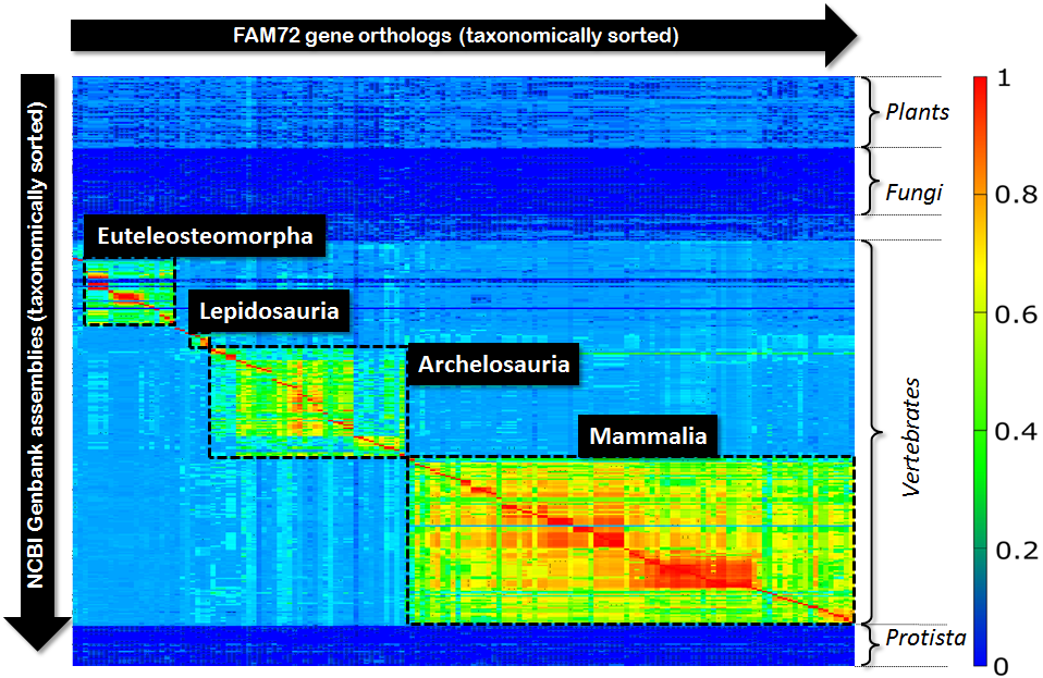
Fig 1.: Klee-diagram for gene FAM72. The color indicates the score for aligning the Exons of a gene ortholog (rows) with respect to a genome (columns). Red indicates a full match and blue indicates no match at all.
First, this diagram tells us that FAM72 occurs in vertebrates exclusively. But second, much more interesting, within vertebrates FAM72 decomposes into four major clusters. Not surprising, these four clusters correspond to the four species groups (Euteleosteomorpha, Lepidosauria, Archelosauria, Mammalia) within vertebrates. But within these clusters we see subclusters as well as tiny clusters sometimes in-between these four major blocks. So, how many clusters are in this diagram altogether? In order to answer this question you typically rely on a standard algorithmic approach like single-linkage-clustering. You define your parameters, thresholds, do your clustering and look, count, compare watching the outcome of the algorithmic process.
Single-linkage-clustering inspects each element of your matrix. So, its runtime is proportional to the overall size of your matrix. But, if we look to the above Klee-diagram, then we can observe that the significant part is only around the red diagonal spanning form top-left to bottom-right within vertebrates. This diagonal will mainly drive the resulting clustering process. And there we have our idea: Instead of inspecting the complete matrix, we only inspect the area around the red-diagonal. Obviously, such a limitation of the inspected area reduces the computational costs significantly. But more interesting, it allows fine tuning with respect to taxonomic cluster alignment that is superior to single-linkage-clustering. This can be explained as follows: Single-linkage-clustering is, due to the inspection of the overall matrix, prone to noise within the vicinity of the central red diagonal. Such noise can result from low quality gene predictions or faulty assemblies. A strong focus on the diagonal itself “blanks out” this noise and the resulting cluster can be better aligned with respect to the basic taxonomy.
Fig. 2 contains two diagrams that shall give an impression of the problem. On the left side you see the clustering of FAM72 for single-linkage clustering. On the right side you see what you get with our proposed clustering algorithm. The clusters are visualized as grey boxes, where the upper part of the box (the part above the red diagonal) is removed for improved visibility.
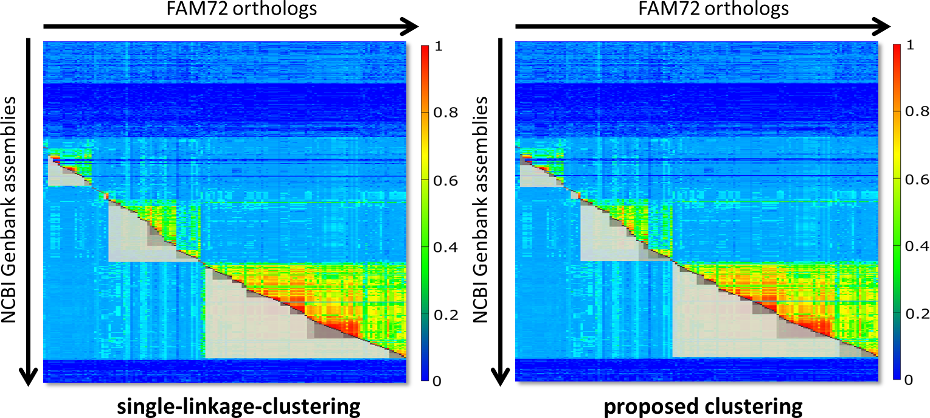
Fig. 2: Comparison of the resulting clusters for classic single-linkage-clustering (left side) and our proposed approach (right side). The thresholds for clustering were hand optimized (25 for single linkage and 65 for our approach), so that the major clusters appear taxonomically as perfect aligned as possible. Single-linkage clustering experiences problems here, as indicated by the gap between Archelosauria and Mammalia or the complete absence of the cluster with Lepidosauria.
Both diagrams of Fig. 2 are fine tuned with the intention that the major clusters are maximally close to the extensions of the respective species groups. The right diagram is almost perfect with respect to this property. But for single-linkage-clustering we run into the following problems: If we switch to a threshold below 25, then Archelosauria and Mammalia are joined in one cluster. For a value above 25 the clusters Archelosauria and Mammalia shrink even more. Further, for a threshold of 25 there is no cluster with Lepidosauria. So, in fact you can not find a threshold that delivers the same perfect clustering like for our approach.
Findings
Seeing this diagram for FAM72, there popped up another question “How does this Klee-diagram for FAM72 look compared to diagrams of other genes? What cluster structures do we have over there?” So, we selected a thousand genes and computed the required alignment matrices (scoring matrices) for all these genes. Generously, our school paid the electric bill and NCBI didn’t blacklist our steadily sucking computational nodes.
FAM72 proved to be rather boring. Its clustering resembles this of many other stable genes, where the clustering reflects more or less the tree of life merely. However, using our fast clustering scheme we were computationally digging for the “crazy” ones. For example genes, where the resulting cluster structure somehow violates the phylogeny of the classic tree of life. Or genes with unusual many clusters compared to the average for all others. Naturally, we found some of these.
Now we present one of our findings, the gene MSTN, where the cluster structure violates the tree of life. But first have a look to Fig. 3.
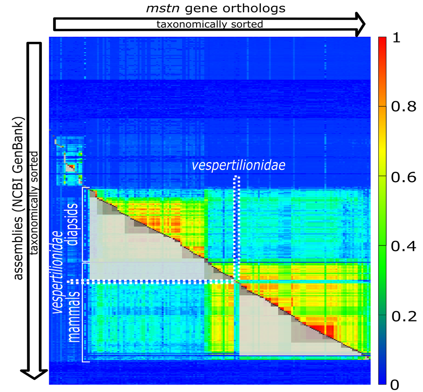
Fig. 3: Clustering for the gene MSTN.
The clustering in Fig. 3 violates the phylogeny of the classic tree of life (we used the NCBI-taxonomy in the context of our work) obviously with vespertilionidae. Batman’s best friends, seem to have a very special form of MSTN. It has mutated so heavily, compared to its evolutionary (taxonomic) neighbors, that the light grey cluster spanning over mammals is broken at this position. If we look into the NCBI-summary of human MSTN, we can find the statement “Mutations in this gene are associated with increased skeletal muscle mass in humans and other mammals.” This allows the assumption that our little flying relatives are quite special with respect to muscle development. Looking into the involved mutations might fulfill bodybuilder’s hottest dreams. But, who knows?
What’s important is that such violations can be found computationally. We simply have to check whether there is a contradiction between taxonomy and clustering. In more detail: We have to check that for all clusters C (the grey boxes cut to half) the extension of C does not simultaneously fully covers one species group and partially covers a neighboring species group. In the above diagram the upper light grey cluster spanning over diapsidis extends into mammals but not fully spans over mammals. This constitutes exactly such kind of previously mentioned violation.
Techniques – Algorithmic Approaches
We will no present some basic techniques and ideas of our proposed form of clustering. First of all there is the question “How do we know the position of the red diagonal?” Now, we have to transform our matrix so that the diagonal becomes a straight 45 degree line in the matrix’s center. This is the case for a matrix with exactly the same taxonomically sorted list of species on X-axis as well as Y-axis. We get such a squared matrix by inserting species not occurring on the Y-axis into the X-axis and, vice versa, inserting species not occurring on the Y-axis into the X-axis, where all freshly created rows and columns are filled with a value that is equal to “no data available”. The matrix of Fig. 4 shows such an extend matrix in the of our FAM72 example. The black areas represent non-existing data.
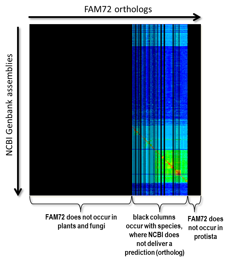
Fig. 4: The alignment scores for the gene FAM72 extended to a squared matrix by inserting required columns and rows. The color black indicates “no data”.
After cluster computation we can remove these blank areas without much reasoning. However, in the context of the clustering process we have to cope appropriately with these blank spots. We do so be cleverly inspecting the environment of a blank spot for available data and inferring data for within on the foundation of what we see around. Details can be found in the publication that belongs to this blog.
In the context of core clustering you can choose among a hierarchical approach and a non-hierarchical one. The hierarchical approach is the computationally more expensive one having a Θ(n log n) complexity, where n is the size of each axis of the matrix (the matrix is squared). Algorithmically it performs clustering by a sequence of hierarchically ordered unions of disjoint sets. The strategy strongly resembles Kruskal’s algorithm for minimum spanning trees. The order used throughout clustering has to be created by stable sorting. With respect to complexity considerations this sorting is the most expensive part of the overall complexity. Because the algorithmic approach is hierarchical we get a dendrogram additional to the clustering.
The non-hierarchical linear-time approach follows a completely different path. Here we do the clustering by a simple right to left scan over the central diagonal, where the cluster construction itself happens on the foundation of a stack (keeping cluster start-positions) in combination with a threshold, which controls cluster ejection. It resembles somehow stack based parsing techniques that we know from the area of syntax analysis. Naturally, such a scan can be done in Θ(n), where n is the dimension of the squared matrix.
In the context of a quality evaluation we could prove that both approaches deliver almost equal clusters. First this might appear a bit surprising. But, if we strip the hierarchic approach its hierarchic behavior, it becomes visible that the stack performs a job equal to the repeated unions of disjoint sets.
Implementation
![]() Clustor is a Java-application that implements the proposed clustering scheme. It has a small GUI, where you can select a matrix (see the program documentation for more info about the matrix format) and set several clustering parameters. The outcome of the clustering can be requested in visualized form, delivering diagrams as shown over here. Further, these diagrams can be stored as PNG-files for further processing.
Clustor is a Java-application that implements the proposed clustering scheme. It has a small GUI, where you can select a matrix (see the program documentation for more info about the matrix format) and set several clustering parameters. The outcome of the clustering can be requested in visualized form, delivering diagrams as shown over here. Further, these diagrams can be stored as PNG-files for further processing.
Clustor is open source and licensed under the GPL.
Download
Source files as well as the executable jar file of the reference implementation can be obtained here:
Clustor Verison 1.0 (zip-file)
The application does not perform alignments. It loads already prepared scoring-matrices that have to be available via the Excel-XML format. Some already prepared Excel-XML files are available for download over here:
Excel-XML Example Scoring Matrices (zip-file)
More info
A more detailed presentation of our clustering approach has been submitted for journal publication. However, if you want to know more just now, please contact waywatcher1(at)web.de or kutzner(at)hanyang.ac.kr for more info.